Using the lazyfmri-package

This notebook shows a couple of functionalities of the lazyfmri-package, including reading in data, plotting + statistics, and deconvolution procedures.

[1]:

from lazyfmri import (
    plotting,
    glm,
    utils,
    fitting,
    dataset,
    preproc
)
import pingouin as pg
import os
import pandas as pd
import matplotlib.pyplot as plt
opj = os.path.join
opd = os.path.dirname

Dataset: Read data

[3]:

data_dir = opj(opd(plotting.__file__), "data")
os.listdir(data_dir)

[3]:

['df_metrics.png',
 'profiles.csv',
 'df_func.png',
 'glms.csv',
 'df_onsets.png',
 'sub-01_ses-1_task-SRF_events.tsv',
 'betas.csv',
 'sub-01_ses-1_task-SRF_bold.mat',
 'sub-01_ses-1_task-SRF_eye.edf',
 'example.png']

[4]:

func = opj(data_dir, "sub-01_ses-1_task-SRF_bold.mat")
tsv = opj(data_dir, "sub-01_ses-1_task-SRF_events.tsv")
edf = opj(data_dir, "sub-01_ses-1_task-SRF_eye.edf")
t = dataset.Dataset(
    func,
    tsv_file=tsv,
    # edf_file=edf,
    verbose=True,
    phase_onset=0,
    ica=True,
    merge=False,
)

DATASET

FUNCTIONAL
Preprocessing /Users/heij/miniconda3/lib/python3.9/site-packages/lazyfmri/data/sub-01_ses-1_task-SRF_bold.mat
 Filtering strategy: 'hp'
 Standardization strategy: 'psc'
 Baseline is 20 seconds, or 190 TRs
 Cutting 0 vols from beginning (also cut from baseline (was 190, now 190 TRs) | 0 vols from end
 DCT-high pass filter [removes low frequencies <0.01 Hz] to correct low-frequency drifts.
 Running FastICA with 5 components
 DCT high-pass filter on components [removes low frequencies <0.2 Hz]
 Regressing out all high-passed components [>0.2 Hz]
 tSNR [before 'ica']: 6.56      | variance: 26.82
 tSNR [after 'ica']:  6.72      | variance: 25.85

EXPTOOLS
Preprocessing /Users/heij/miniconda3/lib/python3.9/site-packages/lazyfmri/data/sub-01_ses-1_task-SRF_events.tsv
 1st 't' @37.13s
 Extracting ['b'] button(s)
 Cutting 37.13s from onsets

DATASET: created

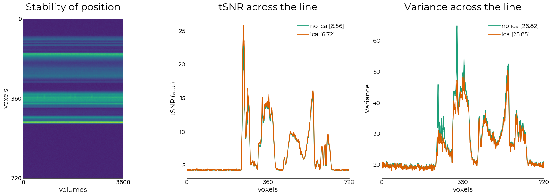
[5]:

t.basic_qa(
    t.ts_corrected,
    run=1,
    make_figure=True
)

 tSNR [before 'ica']: 6.56      | variance: 26.82
 tSNR [after 'ica']:  6.72      | variance: 25.85

[6]:

# preprocessed functional data (high-pass + ICA [5 comps])
t.fetch_fmri().head()

Fetching dataframe from attribute 'df_func_ica'

[6]:

			vox 0	vox 1	vox 2	vox 3	vox 4	vox 5	vox 6	vox 7	vox 8	vox 9	...	vox 710	vox 711	vox 712	vox 713	vox 714	vox 715	vox 716	vox 717	vox 718	vox 719
subject	run	t
01	1	0.000	24.120995	26.884232	-6.523682	-13.212769	-26.410553	5.315056	38.903366	-3.039337	32.551918	-0.393822	...	35.238266	68.940781	-46.369797	-12.008331	2.939903	41.984879	14.404648	10.435143	17.629280	-18.974892
		0.105	60.904526	-4.066513	-5.549294	10.578300	-31.444527	-13.776810	9.944603	-11.358437	31.305672	7.784973	...	29.101364	-1.237228	42.155609	2.658195	33.851700	-17.355743	15.824417	20.952255	28.794029	20.434402
		0.210	-10.842644	-29.055435	15.535713	-36.002487	15.479706	-7.587608	-1.707916	12.058693	-16.157364	-7.403816	...	-18.747169	-31.623734	-4.397873	79.508301	29.455460	-18.974419	-1.437408	45.921638	-24.293541	8.289619
		0.315	-22.451355	-3.198708	1.316246	-10.250626	-12.907562	-26.392105	7.321220	50.494308	0.506996	22.063896	...	-14.635651	-3.495102	5.431557	-13.444511	-14.753075	-8.381844	-13.837997	27.244171	-5.284363	-31.195488
		0.420	-4.934433	1.994728	50.188454	29.976830	4.476112	9.072395	-2.892616	23.413216	-50.936028	16.053589	...	19.833023	1.415779	4.240707	38.267975	15.010330	12.893593	-4.238487	62.481651	-34.293571	-0.052536

5 rows × 720 columns

[7]:

# event onsets
t.df_onsets.head()

[7]:

			onset
subject	run	event_type
01	1	suppr_1	30.016442
		act	48.358001
		act	74.357842
		suppr_1	96.282811
		suppr_1	113.007627

NideconvFitter: deconvolve data

You can either input your entire dataset in the fitter, or select a subset of the dataframe using utils.select_from_df() based on the columns (used indices=[354,360]) or rows/index (expression="index = value"):

[8]:

# select particular run
func = utils.select_from_df(
    t.fetch_fmri(),
    expression="run = 1"
)
func.head()

Fetching dataframe from attribute 'df_func_ica'

[8]:

			vox 0	vox 1	vox 2	vox 3	vox 4	vox 5	vox 6	vox 7	vox 8	vox 9	...	vox 710	vox 711	vox 712	vox 713	vox 714	vox 715	vox 716	vox 717	vox 718	vox 719
subject	run	t
01	1	0.000	24.120995	26.884232	-6.523682	-13.212769	-26.410553	5.315056	38.903366	-3.039337	32.551918	-0.393822	...	35.238266	68.940781	-46.369797	-12.008331	2.939903	41.984879	14.404648	10.435143	17.629280	-18.974892
		0.105	60.904526	-4.066513	-5.549294	10.578300	-31.444527	-13.776810	9.944603	-11.358437	31.305672	7.784973	...	29.101364	-1.237228	42.155609	2.658195	33.851700	-17.355743	15.824417	20.952255	28.794029	20.434402
		0.210	-10.842644	-29.055435	15.535713	-36.002487	15.479706	-7.587608	-1.707916	12.058693	-16.157364	-7.403816	...	-18.747169	-31.623734	-4.397873	79.508301	29.455460	-18.974419	-1.437408	45.921638	-24.293541	8.289619
		0.315	-22.451355	-3.198708	1.316246	-10.250626	-12.907562	-26.392105	7.321220	50.494308	0.506996	22.063896	...	-14.635651	-3.495102	5.431557	-13.444511	-14.753075	-8.381844	-13.837997	27.244171	-5.284363	-31.195488
		0.420	-4.934433	1.994728	50.188454	29.976830	4.476112	9.072395	-2.892616	23.413216	-50.936028	16.053589	...	19.833023	1.415779	4.240707	38.267975	15.010330	12.893593	-4.238487	62.481651	-34.293571	-0.052536

5 rows × 720 columns

[9]:

t.fetch_fmri()

Fetching dataframe from attribute 'df_func_ica'

[9]:

			vox 0	vox 1	vox 2	vox 3	vox 4	vox 5	vox 6	vox 7	vox 8	vox 9	...	vox 710	vox 711	vox 712	vox 713	vox 714	vox 715	vox 716	vox 717	vox 718	vox 719
subject	run	t
01	1	0.000	24.120995	26.884232	-6.523682	-13.212769	-26.410553	5.315056	38.903366	-3.039337	32.551918	-0.393822	...	35.238266	68.940781	-46.369797	-12.008331	2.939903	41.984879	14.404648	10.435143	17.629280	-18.974892
		0.105	60.904526	-4.066513	-5.549294	10.578300	-31.444527	-13.776810	9.944603	-11.358437	31.305672	7.784973	...	29.101364	-1.237228	42.155609	2.658195	33.851700	-17.355743	15.824417	20.952255	28.794029	20.434402
		0.210	-10.842644	-29.055435	15.535713	-36.002487	15.479706	-7.587608	-1.707916	12.058693	-16.157364	-7.403816	...	-18.747169	-31.623734	-4.397873	79.508301	29.455460	-18.974419	-1.437408	45.921638	-24.293541	8.289619
		0.315	-22.451355	-3.198708	1.316246	-10.250626	-12.907562	-26.392105	7.321220	50.494308	0.506996	22.063896	...	-14.635651	-3.495102	5.431557	-13.444511	-14.753075	-8.381844	-13.837997	27.244171	-5.284363	-31.195488
		0.420	-4.934433	1.994728	50.188454	29.976830	4.476112	9.072395	-2.892616	23.413216	-50.936028	16.053589	...	19.833023	1.415779	4.240707	38.267975	15.010330	12.893593	-4.238487	62.481651	-34.293571	-0.052536
		...	...	...	...	...	...	...	...	...	...	...	...	...	...	...	...	...	...	...	...	...	...
		377.475	-12.011627	-27.804131	-4.247818	3.850395	13.434708	-13.325851	-11.991318	48.694641	-14.418465	17.417793	...	11.003410	5.086433	9.591133	2.009270	-1.192749	-31.425163	19.871819	9.320839	-31.430031	-43.894890
		377.580	0.978722	12.072548	1.603668	16.085312	-8.246437	-9.025551	-13.306900	13.437164	21.946548	-9.839020	...	-13.095047	-42.527115	32.514877	-12.019234	20.575027	23.909904	-13.735153	-39.035683	-10.055534	-11.766006
		377.685	-35.623386	9.984329	51.675240	1.970345	40.135155	-20.763428	8.739861	-10.021568	34.045082	0.650864	...	-23.774216	-25.980812	-27.767540	-10.051491	39.635025	14.152061	16.660095	34.088905	18.116859	-3.807968
		377.790	37.096939	-13.449570	17.217300	-12.686440	11.852051	16.513260	3.448265	21.950768	23.538857	-1.577194	...	-10.944649	12.543327	-3.919037	3.668861	4.819633	9.076393	15.658363	-12.369011	-27.114166	-22.759338
		377.895	-14.316536	14.075386	20.446785	-9.932777	25.556366	5.452995	20.317551	32.211632	5.674583	7.165482	...	2.156181	24.890739	-15.975510	27.382568	-13.209038	-3.198730	-20.116196	-11.395653	21.581970	34.095779

3600 rows × 720 columns

[10]:

# select columns
func = utils.select_from_df(
    t.fetch_fmri(),
    indices=(358,363)
)
func.head()

Fetching dataframe from attribute 'df_func_ica'

[10]:

			vox 358	vox 359	vox 360	vox 361	vox 362
subject	run	t
01	1	0.000	-13.839142	-0.588173	-8.102196	-2.139931	4.546173
		0.105	-15.945457	-1.409012	9.016457	-4.400345	-0.167259
		0.210	3.386215	-2.018135	-1.606422	3.617538	-4.278763
		0.315	4.105896	-4.456375	-5.251724	7.006035	1.271133
		0.420	16.345734	-4.209183	-5.079575	0.242401	-9.488388

[11]:

# initialize the fitter
dec = fitting.NideconvFitter(
    func,
    t.fetch_onsets(),
    basis_sets="canonical_hrf_with_time_derivative",
    TR=0.105,
    interval=[-2,16],
    verbose=True,
    conf_intercept=False
)

dec.timecourses_condition()

Selected 'canonical_hrf_with_time_derivative'-basis sets (with 2 regressors)
Adding event 'act' to model
Adding event 'suppr_1' to model
Adding event 'suppr_2' to model
Fitting with 'ols' minimization
Fitting completed
Fetching subject/condition-wise time courses from <nideconv.group_analysis.GroupResponseFitter object at 0x13aa04a90>

[12]:

# average over the voxels and parse into list
evs = utils.get_unique_ids(dec.tc_condition, id="event_type")

tc,se,pr = [],[],[]
for i in evs:
    avg = utils.select_from_df(
        dec.tc_condition,
        expression=f"event_type = {i}"
    )

    pred = utils.select_from_df(
        dec.ev_predictions,
        expression=f"event_type = {i}"
    )

    tc.append(avg.mean(axis=1).values)
    se.append(avg.sem(axis=1).values)
    pr.append(pred.mean(axis=1).values)

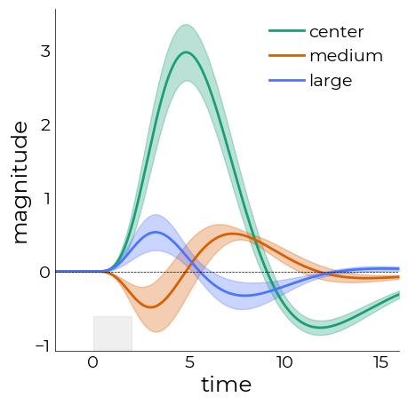
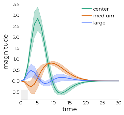
LazyLine: plot simple lines

[13]:

%matplotlib inline

# do some plotting
pl = plotting.LazyLine(
    tc,
    xx=dec.time,
    figsize=(5,5),
    color=["#1B9E77","#D95F02","#4c75ff"],
    error=se,
    line_width=2,
    labels=["center","medium","large"],
    x_label="time",
    y_label="magnitude",
    add_hline=0
)

plotting.add_axvspan(
    pl.axs,
    ymax=0.1
)

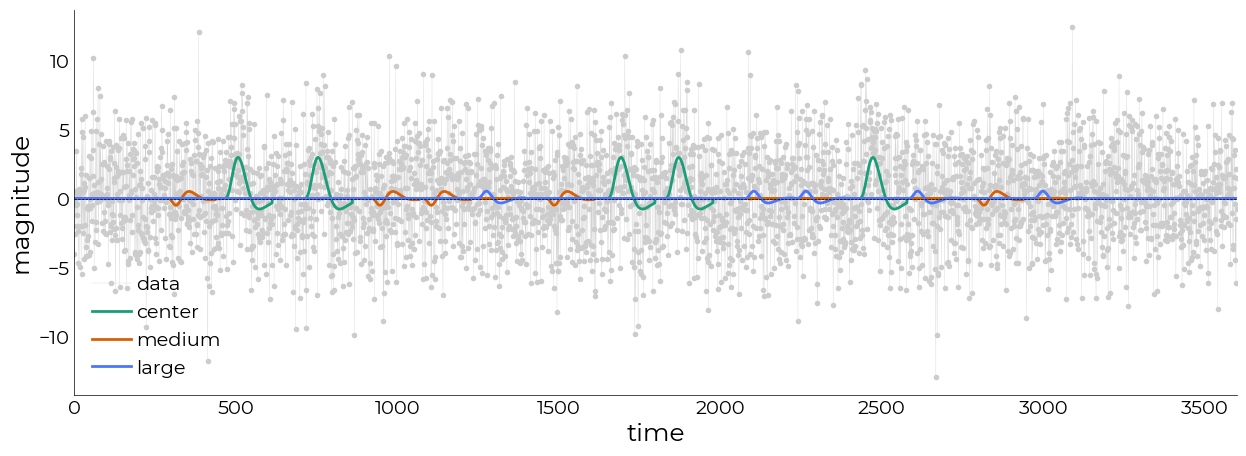
[16]:

%matplotlib inline

# do some plotting
pl = plotting.LazyLine(
    [dec.func.mean(axis=1).values]+pr,
    figsize=(15,5),
    color=["#cccccc","#1B9E77","#D95F02","#4c75ff"],
    line_width=[0.2,2,2,2],
    labels=["data","center","medium","large"],
    x_label="time",
    y_label="magnitude",
    add_hline=0,
    markers=[".", None, None, None]
)

DataFilter: apply filter to entire dataframe

[17]:

%matplotlib inline

filt = preproc.DataFilter(
    dec.func,
    filter_strategy="lp"
)

# initialize the fitter
dec = fitting.NideconvFitter(
    filt.df_filt,
    t.fetch_onsets(),
    basis_sets="canonical_hrf_with_time_derivative",
    TR=0.105,
    interval=[-2,16],
    verbose=True,
    conf_intercept=False
)

dec.timecourses_condition()

# average over the voxels and parse into list
evs = utils.get_unique_ids(dec.tc_condition, id="event_type")

tc,se,pr = [],[],[]
for i in evs:
    avg = utils.select_from_df(
        dec.tc_condition,
        expression=f"event_type = {i}"
    )

    pred = utils.select_from_df(
        dec.ev_predictions,
        expression=f"event_type = {i}"
    )

    tc.append(avg.mean(axis=1).values)
    se.append(avg.sem(axis=1).values)
    pr.append(pred.mean(axis=1).values)


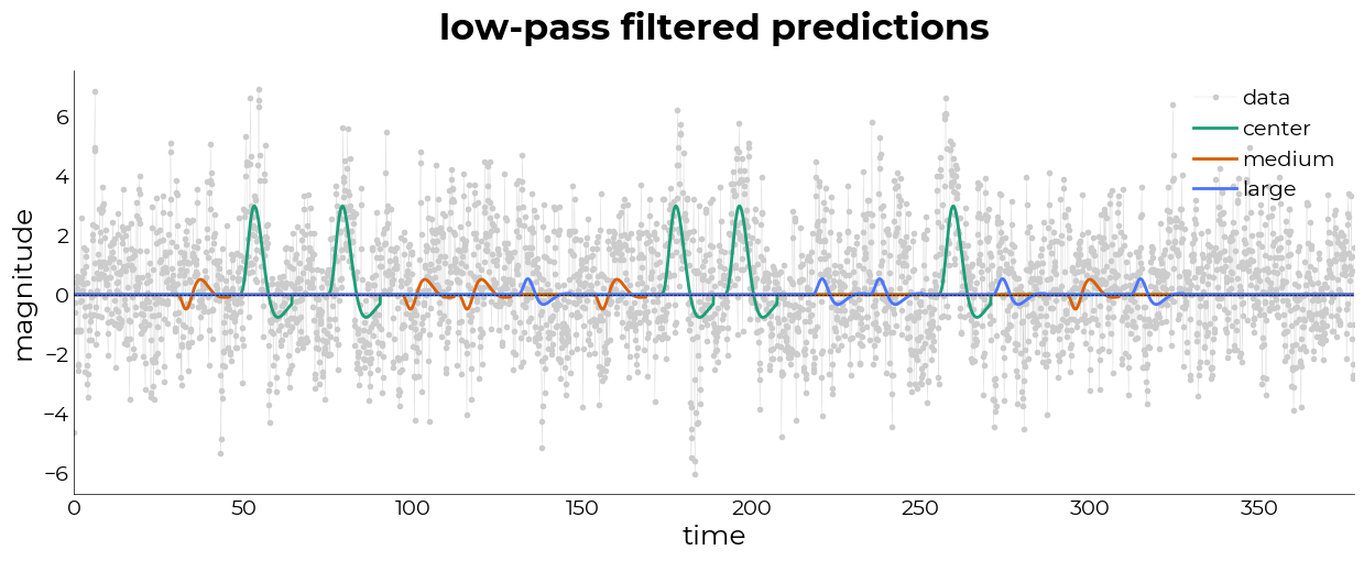
# do some plotting
pl = plotting.LazyLine(
    [dec.func.mean(axis=1).values]+pr,
    xx=utils.get_unique_ids(dec.func, id="t"),
    figsize=(15,5),
    color=["#cccccc","#1B9E77","#D95F02","#4c75ff"],
    line_width=[0.2,2,2,2],
    labels=["data","center","medium","large"],
    x_label="time",
    y_label="magnitude",
    add_hline=0,
    markers=[".", None, None, None],
    title={
        "title": "low-pass filtered predictions",
        "fontweight": "bold"
    }
)

Selected 'canonical_hrf_with_time_derivative'-basis sets (with 2 regressors)
Adding event 'act' to model
Adding event 'suppr_1' to model
Adding event 'suppr_2' to model
Fitting with 'ols' minimization
Fitting completed
Fetching subject/condition-wise time courses from <nideconv.group_analysis.GroupResponseFitter object at 0x13ab71990>

These classes also have the capability to extract relevant information from the deconvolved HRF profiles. The success of the estimation depends on the basis sets used and the quality of the data.

[18]:

dec.parameters_for_tc_subjects()
dec.pars_subjects.head()

Deriving parameters from <lazyfmri.fitting.NideconvFitter object at 0x13a836980> with 'HRFMetrics'

[18]:

				magnitude	magnitude_ix	fwhm	fwhm_obj	time_to_peak	half_rise_time	half_max	rise_slope	onset_time	positive_area	undershoot	1st_deriv_magnitude	1st_deriv_time_to_peak	2nd_deriv_magnitude	2nd_deriv_time_to_peak
subject	event_type	run	vox
01	act	1	vox 358	2.467425	1485	4.364710	<lazyfmri.fitting.FWHM object at 0x13ac59720>	5.798530	3.805654	1.233713	1.005427	2.585273	10.658189	2.815127	-0.115784	1.192934	-0.174174	0.741302
			vox 359	2.800170	1206	4.145993	<lazyfmri.fitting.FWHM object at 0x13ac5a1d0>	4.333352	2.446804	1.400085	1.182195	1.263848	11.574219	3.700148	1.241342	2.421793	0.918949	1.313719
			vox 360	2.781102	1197	4.108069	<lazyfmri.fitting.FWHM object at 0x13ac5ad70>	4.286088	2.419824	1.390551	1.186402	1.249143	11.390945	3.689496	1.246229	2.395535	0.932820	1.297964
			vox 361	2.950976	1328	4.450755	<lazyfmri.fitting.FWHM object at 0x13ac58f40>	4.974039	2.909469	1.475488	1.110632	1.579637	13.111810	3.737924	1.166981	2.920689	0.735578	1.670823
			vox 362	4.426424	1316	4.438020	<lazyfmri.fitting.FWHM object at 0x13ac5b4c0>	4.911021	2.855035	2.213212	1.677232	1.534549	19.605648	5.632660	1.762065	2.857670	1.125011	1.618308

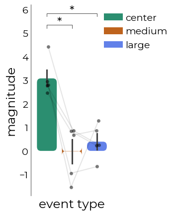
LazyBar: barplots including significance bars

[19]:

# which we can then flop into a LazyBar-object
br = plotting.LazyBar(
    dec.pars_subjects,
    figsize=(2,5),
    x="event_type",
    y="magnitude",
    sns_offset=4,
    fancy=True,
    x_label="event type",
    y_label="magnitude",
    connect=True,
    points_color="k",
    points_alpha=0.5,
    palette=["#1B9E77","#D95F02","#4c75ff"],
    lbl_legend=["center","medium","large"],
    bar_legend=True,
    bbox_to_anchor=(0.8,1)
)

# add the stats
normality = pg.normality(br.data[br.y])
is_normal = normality["normal"][0]

aov = glm.ANOVA(
    data=br.data,
    dv=br.y,
    between=br.x,
    # test="test",
    parametric=is_normal,
    posthoc_kw={
        "effsize": "cohen",
        "test": "test",
        "paired": True,
        "subject": "vox",
        "padjust": "holm"
    }
)

aov.plot_bars(
    axs=br.ff,
    ast_frac=0,
    y_pos=1.15,
    line_separate_factor=-0.075
)

print("\n", normality)
print("\n", aov.ano)
print("\n", aov.posthoc_sorted)


                   W      pval  normal
magnitude  0.961831  0.724179    True

        Source  ddof1  ddof2          F     p-unc      np2
0  event_type      2     12  17.535832  0.000274  0.74507

      Contrast        A        B  Paired  Parametric         T  dof  \
1  event_type      act  suppr_2    True        True  5.036345  4.0
0  event_type      act  suppr_1    True        True  6.173944  4.0
2  event_type  suppr_1  suppr_2    True        True -0.784411  4.0

  alternative     p-unc    p-corr p-adjust   BF10     cohen  distances
1   two-sided  0.007301  0.014602     holm  8.849  3.556338          2
0   two-sided  0.003496  0.010487     holm   15.1  3.202325          1
2   two-sided  0.476649  0.476649     holm  0.505 -0.438658          1

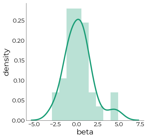
LazyHist: plot histograms

[111]:

glms = pd.read_csv(opj(data_dir,"glms.csv"), usecols=lambda column: not column.startswith("Unnamed"))

[112]:

color = "#1B9E77"
hist = plotting.LazyHist(
    utils.multiselect_from_df(
        glms,
        expression=[
            "preproc = corr",
            "method = norm",
            "model = camel_deriv"
        ]
    )["beta"],
    figsize=(5,5),
    kde=True,
    color=color,
    kde_kwargs={
        "linewidth": 3,
    },
    hist_kwargs={
        "alpha": 0.3,
        "fc": color
    },
    x_label="beta",
    y_label="density"
)

ParameterFitter: estimate parameters from double-gamma HRF

The double-gamma HRF can also be described by a set of parameters (7), rather than a set of basissets that is used for deconvolution. Similar to pRF fitting, this becomes an optimization procedure. This class iteratively assesses the best combination of parameters that mimimizes the error between the prediction the HRF generates and the actual data.

[ ]:

par = fitting.ParameterFitter(
    filt.df_filt,
    t.fetch_onsets()
)

par.fit(
    osf=1, # higher values slow down the convolution process, but are more accurate wrt the onsets
    verbose=True,
    n_jobs=None # "None" sets the number of jobs to the number of input voxels.. be careful with a large number of voxels. Use an integer value to constrain the process to a certain number of jobs.
)

[Parallel(n_jobs=5)]: Using backend LokyBackend with 5 concurrent workers.
[Parallel(n_jobs=5)]: Done   2 out of   5 | elapsed:   24.7s remaining:   37.1s
[Parallel(n_jobs=5)]: Done   5 out of   5 | elapsed:   49.8s finished
[Parallel(n_jobs=5)]: Using backend LokyBackend with 5 concurrent workers.
[Parallel(n_jobs=5)]: Done   2 out of   5 | elapsed:   21.9s remaining:   32.9s
[Parallel(n_jobs=5)]: Done   5 out of   5 | elapsed:   45.0s finished
[Parallel(n_jobs=5)]: Using backend LokyBackend with 5 concurrent workers.
[Parallel(n_jobs=5)]: Done   2 out of   5 | elapsed:   20.6s remaining:   30.8s
[Parallel(n_jobs=5)]: Done   5 out of   5 | elapsed:   35.8s finished

[98]:

# from this, we can extract estimates of individual parameter estimates that generate the full HRF
par.estimates.head()

[98]:

				a1	a2	b1	b2	c	d1	d2
subject	event_type	run	vox
01	act	1	vox 358	7.999986	10.000003	1.158610	0.800000	0.488982	4.907072	14.959780
			vox 359	4.911836	10.564334	1.076591	0.800003	0.402760	9.999969	13.874413
			vox 360	4.176546	11.129979	1.199997	0.800005	0.365645	9.651971	14.378838
			vox 361	4.000091	13.686921	1.199999	0.800004	0.416347	2.082332	13.708682
			vox 362	6.042051	12.164910	0.869612	0.800002	0.445467	9.999975	14.638781

[99]:

# similar to deconvolution, we can call this function to extract relevant parameters from the HRF generated with the estimates
par.parameters_for_tc_subjects()
par.pars_subjects.head()

[99]:

				magnitude	magnitude_ix	fwhm	fwhm_obj	time_to_peak	half_rise_time	half_max	rise_slope	onset_time	positive_area	undershoot	1st_deriv_magnitude	1st_deriv_time_to_peak	2nd_deriv_magnitude	2nd_deriv_time_to_peak
subject	event_type	run	vox
01	act	1	vox 358	2.350515	7	4.289343	<lazyplot.fitting.FWHM object at 0x138ac9850>	7.241379	5.075891	1.171200	0.753576	3.521701	9.092618	5.176764	0.761063	5.172414	0.259572	4.137931
			vox 359	2.842579	5	4.125753	<lazyplot.fitting.FWHM object at 0x13802b690>	5.172414	2.697976	1.421168	NaN	NaN	11.232870	2.977184	1.029912	3.103448	0.400542	1.034483
			vox 360	2.753171	4	4.265000	<lazyplot.fitting.FWHM object at 0x138019350>	4.137931	2.507538	1.375451	NaN	NaN	11.225525	3.470401	0.925612	2.068966	0.392741	1.034483
			vox 361	2.870323	5	5.245565	<lazyplot.fitting.FWHM object at 0x137febdd0>	5.172414	2.483631	1.434844	NaN	NaN	14.913531	1.665688	0.947662	2.068966	0.389894	1.034483
			vox 362	4.602402	5	4.329915	<lazyplot.fitting.FWHM object at 0x139e6cb50>	5.172414	3.065600	2.298418	1.633259	1.658337	19.311170	3.876998	1.631864	3.103448	0.632060	2.068966

[105]:

# the output from the parameter fitter is the same as those from deconvolution using nideconv, so we can use the same code to generate plots
evs = utils.get_unique_ids(par.tc_condition, id="event_type")

tc1,se1,pr1 = [],[],[]
for i in evs:
    avg = utils.select_from_df(
        par.tc_condition,
        expression=f"event_type = {i}"
    )

    pred = utils.select_from_df(
        par.ev_predictions,
        expression=f"event_type = {i}"
    )

    tc1.append(avg.mean(axis=1).values)
    se1.append(avg.sem(axis=1).values)
    pr1.append(pred.mean(axis=1).values)

[107]:

%matplotlib inline

# do some plotting
pl = plotting.LazyLine(
    tc1,
    xx=utils.get_unique_ids(par.tc_condition, id="time"),
    figsize=(5,5),
    color=["#1B9E77","#D95F02","#4c75ff"],
    error=se1,
    line_width=2,
    labels=["center","medium","large"],
    x_label="time",
    y_label="magnitude",
    add_hline=0
)

plotting.add_axvspan(
    pl.axs,
    ymax=0.1
)

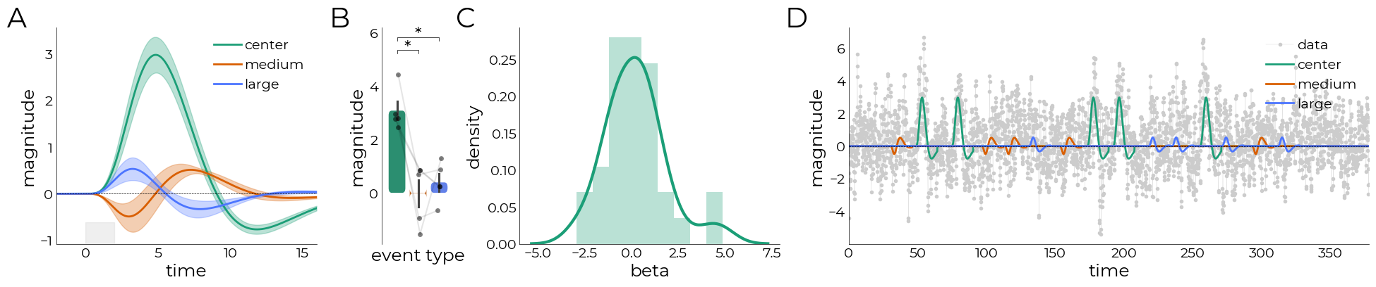
Summary Figure

[113]:

fig,axs = plt.subplots(
    ncols=4,
    width_ratios=[0.2,0.05,0.2,0.4],
    figsize=(24,4),
    gridspec_kw={
        "wspace": 0.25
    }
)

# LazyLine
pl = plotting.LazyLine(
    tc,
    xx=dec.time,
    axs=axs[0],
    color=["#1B9E77","#D95F02","#4c75ff"],
    error=se,
    line_width=2,
    labels=["center","medium","large"],
    x_label="time",
    y_label="magnitude",
    add_hline=0
)

plotting.add_axvspan(
    pl.axs,
    ymax=0.1
)

# LazyBar
br = plotting.LazyBar(
    dec.pars_subjects,
    axs=axs[1],
    x="event_type",
    y="magnitude",
    sns_offset=4,
    fancy=True,
    x_label="event type",
    y_label="magnitude",
    connect=True,
    points_color="k",
    points_alpha=0.5,
    palette=["#1B9E77","#D95F02","#4c75ff"],
    lbl_legend=["center","medium","large"],
)

# add the stats
normality = pg.normality(br.data[br.y])
is_normal = normality["normal"][0]

aov = glm.ANOVA(
    data=br.data,
    dv=br.y,
    between=br.x,
    # test="test",
    parametric=is_normal,
    posthoc_kw={
        "effsize": "cohen",
        "test": "test",
        "paired": True,
        "subject": "vox",
        "padjust": "holm"
    }
)

aov.plot_bars(
    axs=br.ff,
    ast_frac=-0.015,
    y_pos=1.15,
    line_separate_factor=-0.075
)

# LazyHist
plotting.LazyHist(
    utils.multiselect_from_df(
        glms,
        expression=[
            "preproc = corr",
            "method = norm",
            "model = camel_deriv"
        ]
    )["beta"],
    axs=axs[2],
    kde=True,
    color="#1B9E77",
    kde_kwargs={
        "linewidth": 3,
    },
    hist_kwargs={
        "alpha": 0.3,
        "fc": "#1B9E77"
    },
    x_label="beta",
    y_label="density"
)

# Timecourse (predictions)
pl = plotting.LazyLine(
    [dec.func.mean(axis=1).values]+pr,
    xx=utils.get_unique_ids(dec.func, id="t"),
    axs=axs[-1],
    color=["#cccccc","#1B9E77","#D95F02","#4c75ff"],
    line_width=[0.2,2,2,2],
    labels=["data","center","medium","large"],
    x_label="time",
    y_label="magnitude",
    add_hline=0,
    markers=[".", None, None, None],
)

plotting.fig_annot(
    fig,
    x0_corr=-0.7,
    x_corr=[-0.8,-0.9,-0.9],
    y=1
)

# fig.savefig(
#     opj(data_dir, "example.png"),
#     bbox_inches="tight",
#     dpi=300,
#     facecolor="white"
# )